将行和列合并，以创建一个2x2表格来进行费雪精确检验。

Question

我需要使用Python对以下交叉表ct执行独立性检验。

由于某些值小于5，我无法执行卡方独立性检验。因此，我需要执行Fisher精确检验。

然而，在Scipy中，Fisher精确检验的实现只支持2x2表格，所以我采用了以下解决方案：

from scipy.stats import fisher_exact

# 将行和列合并以创建一个2x2表格
table_2x2 = np.array([[ct[1][4] + ct[2][4] + ct[1][3] + ct[2][3], ct[3][4] + ct[4][4] + ct[3][3] + ct[4][3]],
                      [ct[1][2] + ct[2][2] + ct[1][1] + ct[2][1], ct[3][2] + ct[4][2] + ct[3][1] + ct[4][1]]])

# 对2x2表格执行Fisher精确检验
odds_ratio, p_value = fisher_exact(table_2x2)

# 显示结果
print(f'优势比(Odds Ratio): {odds_ratio}')
print(f'P值(P-value): {p_value}')

这个解决方案是否有效？如果不是，您是否有其他在Python中实现此功能的建议？

Dogbert · Answer

若接受随机化置换检验，您可以利用scipy.stats.permutation_test自行创建检验方法。我们将采用与scipy.stats.chi2_contingency相同的检验统计量，但零假设将类似于Fisher确切检验。

首先，加载所需库并设置示例列联表数据：

import numpy as np
from scipy import stats

# 示例列联表
table = np.asarray([[20, 49, 25, 4],
                    [35, 54, 43, 12],
                    [27, 44, 29, 8],
                    [7, 20, 16, 4]])

# 首先进行卡方检验作为验证步骤
chi2_ref = stats.chi2_contingency(table)

# 将列联表转换为配对样本
def untab(table):
    x = []
    y = []
    m, n = table.shape
    for i in range(m):
        for j in range(n):
            count = table[i, j]
            x += [i] * count
            y += [j] * count
    return np.asarray(x), np.asarray(y)

x_data, y_data = untab(table)

# 定义用于计算卡方统计量的函数
def statistic(x_sample):
    # 根据给定的一个样本，计算卡方统计量
    # permutation_test将会传递x样本的随机排列，
    # 这个函数会为每个排列计算统计量，从而得到在零假设下（即无关联）统计量的分布
    table_permuted = stats.contingency.crosstab(x_sample, y_data).count
    return stats.chi2_contingency(table_permuted).statistic

# 执行随机化置换检验，这里选择备择假设为“右侧检验”
perm_test_result = stats.permutation_test((x_data,), statistic, alternative='greater', 
                                         permutation_type='pairings')

print(perm_test_result.pvalue, chi2_ref.pvalue)  # 输出：0.6592 0.6500840391351904

# 比较随机化置换检验的p值与卡方检验的p值，两者接近一致

# 绘制随机化置换检验的零分布直方图，并与相应的卡方分布曲线进行比较
import matplotlib.pyplot as plt
plt.hist(perm_test_result.null_distribution, bins=30, density=True, label='归一化直方图')

# 计算卡方检验的自由度
df = table.size - sum(table.shape) + table.ndim - 1
chi2_dist = stats.chi2(df)
x_values = np.linspace(0, 40, 300)
plt.plot(x_values, chi2_dist.pdf(x_values), label='卡方分布')

plt.legend()
plt.show()

# 结果表明，尽管原表格中存在一些小计数项，但在零假设下随机化置换检验的统计量分布与具有适当自由度的卡方分布非常相似。

为了深入了解该检验背后的理论（或直观解释），请参阅SciPy教程关于《重采样与蒙特卡洛方法》的部分，特别是其中关于相关样本置换检验的2c部分，可参考资源：https://nbviewer.org/github/scipy/scipy-cookbook/blob/main/ipython/ResamplingAndMonteCarloMethods/resampling_tutorial_2c.ipynb 。

Bite code · Answer

除了使用置换检验之外，还可以执行一种稍微概念上更简单的蒙特卡洛检验。以下是具体实现方法：

首先，我们导入所需的库，并设定一个示例列联表数据：

import numpy as np
from scipy import stats
import matplotlib.pyplot as plt

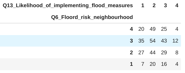
# 示例列联表数据
table = np.asarray([[20, 49, 25, 4],
                    [35, 54, 43, 12],
                    [27, 44, 29, 8],
                    [7, 20, 16, 4]])

# 在零假设（即无关联性）下获取列联表分布
row_totals, col_totals = stats.contingency.margins(table)
null_dist = stats.random_table(row_totals.ravel(), col_totals.ravel())

# 蒙特卡洛零分布：在零假设下随机抽样列联表并计算统计量
n_simulations = 9999
monte_carlo_null_distribution = np.empty(n_simulations, dtype=float)
for i in range(n_simulations):
    resampled_table = stats.chi2_contingency(null_dist.rvs())
    monte_carlo_null_distribution[i] = resampled_table.statistic

# 将观察到的统计量与蒙特卡洛零分布进行比较
observed_chi2 = stats.chi2_contingency(table)
extreme_count = (monte_carlo_null_distribution >= observed_chi2.statistic).sum()
pvalue_mc = (extreme_count + 1) / (n_simulations + 1)  # 0.6534

# 绘制蒙特卡洛零分布和渐近逼近分布
plt.hist(monte_carlo_null_distribution, bins=30, density=True, label='蒙特卡洛')
degrees_of_freedom = table.size - sum(table.shape) + table.ndim - 1
asymptotic_dist = stats.chi2(degrees_of_freedom)
x_axis = np.linspace(0, 40, 300)
plt.plot(x_axis, asymptotic_dist.pdf(x_axis), label='渐近')
plt.legend()
plt.title("卡方检验的零分布")

# 显示图片（对应于WsVk3.png）
# （由于无法实际显示图片，请参照用户上传的WsVk3.png图表）

# 接下来分析临界阈值附近的保守性和安全性
ecdf = stats.ecdf(monte_carlo_null_distribution)
quantiles = ecdf.sf.quantiles[::-1]
prob_mc = ecdf.sf.probabilities[::-1]
prob_asymp = asymptotic_dist.sf(quantiles)
plt.plot(prob_mc, prob_asymp)
plt.xlabel("蒙特卡洛零分布生存概率")
plt.ylabel("渐近零分布生存概率")
plt.plot([0, 1], [0, 1], '--')
plt.xlim(0, 0.1)
plt.ylim(0, 0.1)

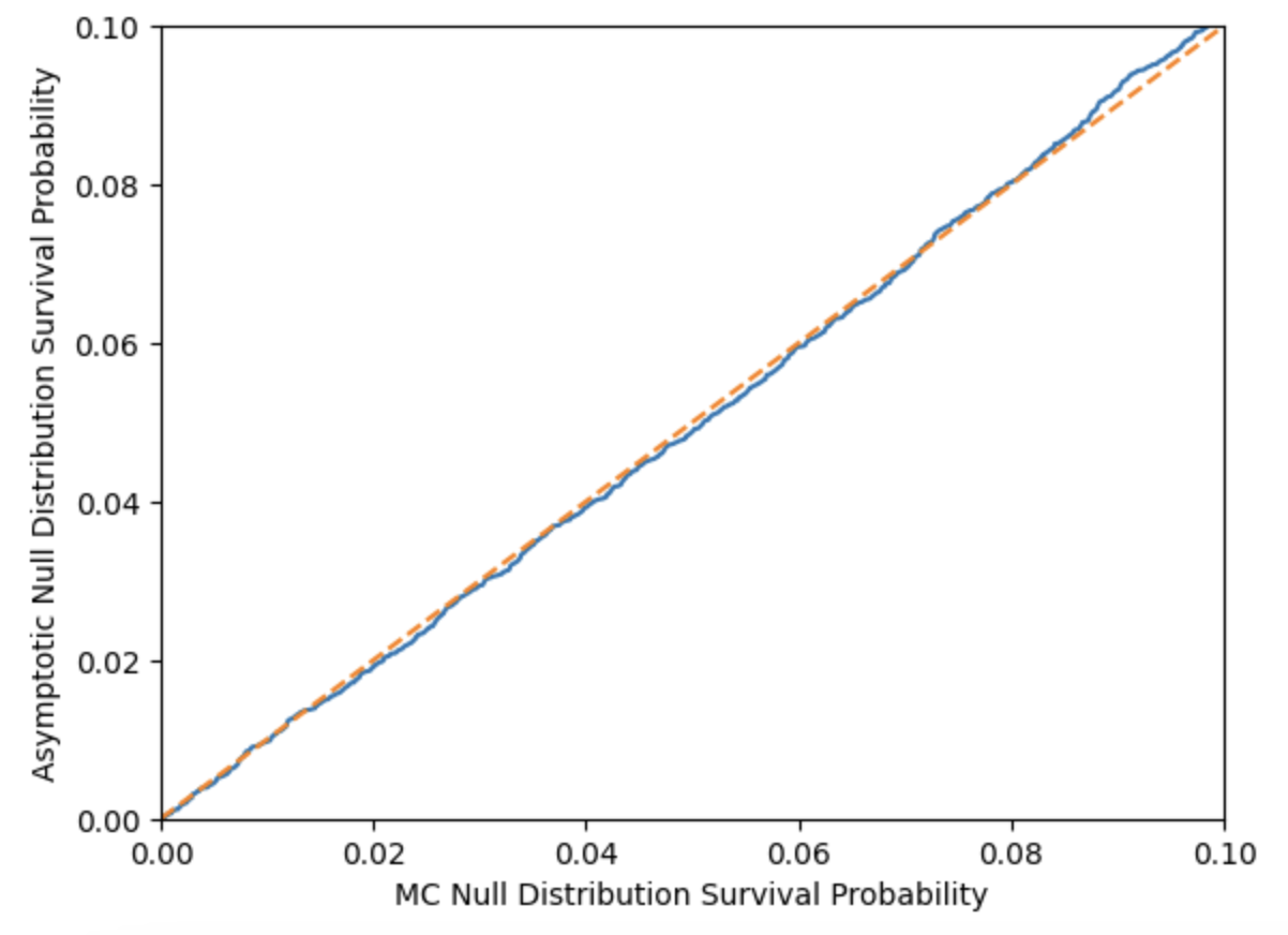
它们之间的匹配度非常高，因此至少对于这个列联表来说，采用渐进卡方检验是相当可靠的。